Visualization

Presenting the results using fancy plots is an important part of solving optimization problems. In this part, we use the Plots.jl package which can be installed via de Pkg prompt within Julia:

Type ] and then:

pkg> add Plots

Or:

julia> import Pkg; Pkg.add("Plots")

Once Plots is installed on your Julia distribution, you will be able to reproduce the following examples.

Assume you want to solve the following minimization problem.

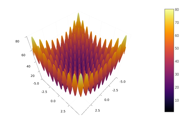
Minimize:

\[f(x) = 10D + \sum_{i=1}^{D} x_i^2 - 10\cos(2\pi x_i)\]

where $x\in[-5, 5]^{D}$, i.e., $-5 \leq x_i \leq 5$ for $i=1,\ldots,D$. $D$ is the dimension number, assume $D=10$.

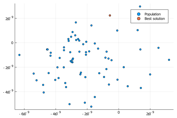
Population Distribution

Let's solve the above optimization problem and plot the resulting population (projecting two specific dimensions).

using Metaheuristics
using Plots
gr()


# objective function
f(x) = 10length(x) + sum( x.^2 - 10cos.(2π*x)  )

# number of variables (dimension)
D = 10

# bounds
bounds = [-5ones(D) 5ones(D)]'

# Common options
options = Options(seed=1)

# Optimizing
result = optimize(f, bounds, ECA(options=options))

# positions in matrix NxD 
X = positions(result)

scatter(X[:,1], X[:,2], label="Population")

x = minimizer(result)
scatter!(x[1:1], x[2:2], label="Best solution")


# (optional) save figure
savefig("final-population.png")

If your optimization problem is scalable, then you also can plot level curves. In this case, let's assume that $D=2$.

using Metaheuristics
using Plots
gr()


# objective function
f(x) = 10length(x) + sum( x.^2 - 10cos.(2π*x)  )

# number of variables (dimension)
D = 2

# bounds
bounds = [-5ones(D) 5ones(D)]'

# Common options
options = Options(seed=1)

# Optimizing
result = optimize(f, bounds, ECA(options=options))

# positions in matrix NxD 
X = positions(result)

xy = range(-5, 5, length=100)
contour(xy, xy, (a,b) -> f([a, b]))

scatter!(X[:,1], X[:,2], label="Population")

x = minimizer(result)
scatter!(x[1:1], x[2:2], label="Best solution")


# (optional) save figure
savefig("final-population-contour.png")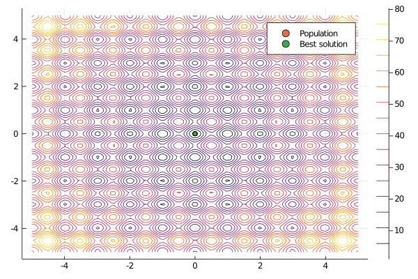

Objective Function Values

Metaheuristics.jl implements some methods to obtain the objective function values (fitness) from the solutions in the resulting population. One of the most useful methods is fvals. In this case, let's use PSO.

using Metaheuristics
using Plots
gr()


# objective function
f(x) = 10length(x) + sum( x.^2 - 10cos.(2π*x)  )

# number of variables (dimension)
D = 10

# bounds
bounds = [-5ones(D) 5ones(D)]'

# Common options
options = Options(seed=1)

# Optimizing
result = optimize(f, bounds, PSO(options=options))

f_values = fvals(result)
plot(f_values)

# (optional) save figure
savefig("fvals.png")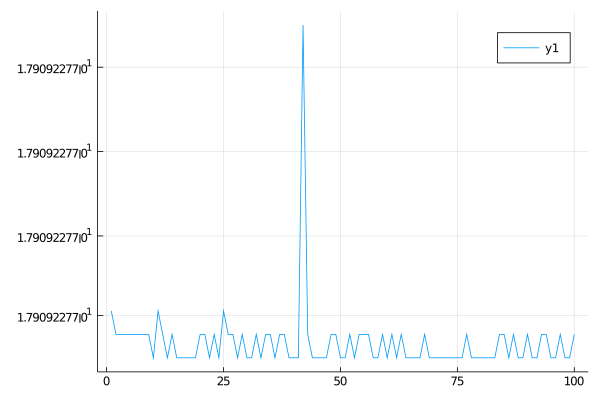

Convergence

Sometimes, it is useful to plot the convergence plot at the end of the optimization process. To do that, it is necessary to set store_convergence = true in Options. Metaheuristics implements a method called convergence.

using Metaheuristics
using Plots
gr()


# objective function
f(x) = 10length(x) + sum( x.^2 - 10cos.(2π*x)  )

# number of variables (dimension)
D = 10

# bounds
bounds = [-5ones(D) 5ones(D)]'

# Common options
options = Options(seed=1, store_convergence = true)

# Optimizing
result = optimize(f, bounds, ECA(options=options))

f_calls, best_f_value = convergence(result)

plot(xlabel="f calls", ylabel="fitness", title="Convergence")
plot!(f_calls, best_f_value, label="ECA")

# (optional) save figure
savefig("convergence.png")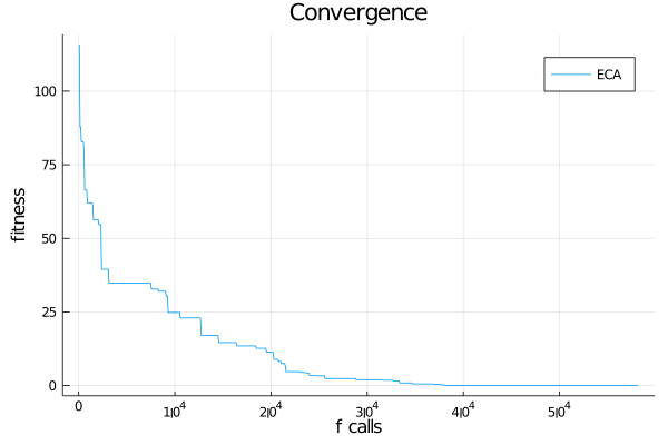

Animate convergence

Also, you can plot the population and convergence in the same figure.

Single-Objective Problem

using Metaheuristics
using Plots
gr()


# objective function
f(x) = 10length(x) + sum( x.^2 - 10cos.(2π*x)  )

# number of variables (dimension)
D = 10

# bounds
bounds = [-5ones(D) 5ones(D)]'

# Common options
options = Options(seed=1, store_convergence = true)

# Optimizing
result = optimize(f, bounds, ECA(options=options))

f_calls, best_f_value = convergence(result)

animation = @animate for i in 1:length(result.convergence)
    l = @layout [a b]
    p = plot( layout=l)

    X = positions(result.convergence[i])
    scatter!(p[1], X[:,1], X[:,2], label="", xlim=(-5, 5), ylim=(-5,5), title="Population")
    x = minimizer(result.convergence[i])
    scatter!(p[1], x[1:1], x[2:2], label="")

    # convergence
    plot!(p[2], xlabel="Generation", ylabel="fitness", title="Gen: $i")
    plot!(p[2], 1:length(best_f_value), best_f_value, label=false)
    plot!(p[2], 1:i, best_f_value[1:i], lw=3, label=false)
    x = minimizer(result.convergence[i])
    scatter!(p[2], [i], [minimum(result.convergence[i])], label=false)
end

# save in different formats
# gif(animation, "anim-convergence.gif", fps=30)
mp4(animation, "anim-convergence.mp4", fps=30)

Multi-Objective Problem

import Metaheuristics: optimize, SMS_EMOA, TestProblems, pareto_front, Options
import Metaheuristics.PerformanceIndicators: Δₚ
using Plots; gr()

# get test function
f, bounds, pf = TestProblems.ZDT6();

# optimize using SMS-EMOA
result = optimize(f, bounds, SMS_EMOA(N=70,options=Options(iterations=500,seed=0, store_convergence=true)))

# true pareto front
B = pareto_front(pf)
# error to the true front
err = [ Δₚ(r.population, pf) for r in result.convergence]
# generate plots
a = @animate for i in 1:5:length(result.convergence)
    A = pareto_front(result.convergence[i])

    p = plot(B[:, 1], B[:,2], label="True Pareto Front", lw=2,layout=(1,2), size=(850, 400))
    scatter!(p[1], A[:, 1], A[:,2], label="SMS-EMOA", markersize=4, color=:black, title="ZDT6")
    plot!(p[2], eachindex(err), err, ylabel="Δₚ", legend=false)
    plot!(p[2], 1:i, err[1:i], title="Generation $i")
    scatter!(p[2], [i], err[i:i])
end

# save animation
gif(a, "ZDT6.gif", fps=20)

Pareto Front

import Metaheuristics: optimize, NSGA2, TestProblems, pareto_front, Options
using Plots; gr()

f, bounds, solutions = TestProblems.ZDT3();

result = optimize(f, bounds, NSGA2(options=Options(seed=0)))

A = pareto_front(result)
B = pareto_front(solutions)

scatter(A[:, 1], A[:,2], label="NSGA-II")
plot!(B[:, 1], B[:,2], label="Parento Front", lw=2)
savefig("pareto.png")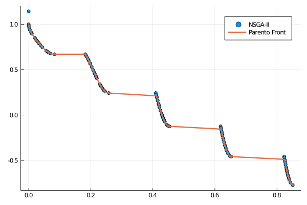

Live Plotting

The optimize function has a keyword parameter named logger that contains a function pointer. Such function will receive the State at the end of each iteration in the main optimization loop.

import Metaheuristics: optimize, NSGA2, TestProblems, pareto_front, Options, fvals
using Plots; gr()

f, bounds, solutions = TestProblems.ZDT3();
pf = pareto_front(solutions)

logger(st) = begin
    A = fvals(st)
    scatter(A[:, 1], A[:,2], label="NSGA-II", title="Gen: $(st.iteration)")
    plot!(pf[:, 1], pf[:,2], label="Parento Front", lw=2)
    gui()
    sleep(0.1)
end

result = optimize(f, bounds, NSGA2(options=Options(seed=0)), logger=logger)