Performance Indicators

Metaheuristics.jl includes performance indicators to assess evolutionary optimization algorithms performance.

Available indicators:

Performance Indicators

Performance Indicators in Julia

Minimization is always assumed here.

Note that in Metaheuristics.jl, minimization is always assumed. Therefore these indicators have been developed for minimization problems.

Metaheuristics.PerformanceIndicators — Module

PerformanceIndicators

This module includes performance indicators to assess evolutionary multi-objective optimization algorithms.

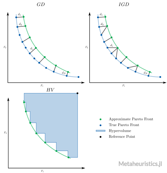
gd Generational Distance.
igd Inverted Generational Distance.
gd_plus Generational Distance plus.
igd_plus Inverted Generational Distance plus.
covering Covering indicator (C-metric).
hypervolume Hypervolume indicator.

Example

julia> import Metaheuristics: PerformanceIndicators, TestProblems

julia> A = [ collect(1:3) collect(1:3) ]
3×2 Array{Int64,2}:
 1  1
 2  2
 3  3

julia> B = A .- 1
3×2 Array{Int64,2}:
 0  0
 1  1
 2  2

julia> PerformanceIndicators.gd(A, B)
0.47140452079103173

julia> f, bounds, front = TestProblems.get_problem(:ZDT1);

julia> front
                          F space
         ┌────────────────────────────────────────┐ 
       1 │⠁⠀⠀⠀⠀⠀⠀⠀⠀⠀⠀⠀⠀⠀⠀⠀⠀⠀⠀⠀⠀⠀⠀⠀⠀⠀⠀⠀⠀⠀⠀⠀⠀⠀⠀⠀⠀⠀⠀⠀│ 
         │⠄⠀⠀⠀⠀⠀⠀⠀⠀⠀⠀⠀⠀⠀⠀⠀⠀⠀⠀⠀⠀⠀⠀⠀⠀⠀⠀⠀⠀⠀⠀⠀⠀⠀⠀⠀⠀⠀⠀⠀│ 
         │⠈⠄⠀⠀⠀⠀⠀⠀⠀⠀⠀⠀⠀⠀⠀⠀⠀⠀⠀⠀⠀⠀⠀⠀⠀⠀⠀⠀⠀⠀⠀⠀⠀⠀⠀⠀⠀⠀⠀⠀│ 
         │⠀⠈⢆⠀⠀⠀⠀⠀⠀⠀⠀⠀⠀⠀⠀⠀⠀⠀⠀⠀⠀⠀⠀⠀⠀⠀⠀⠀⠀⠀⠀⠀⠀⠀⠀⠀⠀⠀⠀⠀│ 
         │⠀⠀⠀⠢⡀⠀⠀⠀⠀⠀⠀⠀⠀⠀⠀⠀⠀⠀⠀⠀⠀⠀⠀⠀⠀⠀⠀⠀⠀⠀⠀⠀⠀⠀⠀⠀⠀⠀⠀⠀│ 
         │⠀⠀⠀⠀⠈⠢⡀⠀⠀⠀⠀⠀⠀⠀⠀⠀⠀⠀⠀⠀⠀⠀⠀⠀⠀⠀⠀⠀⠀⠀⠀⠀⠀⠀⠀⠀⠀⠀⠀⠀│ 
         │⠀⠀⠀⠀⠀⠀⠉⠢⡄⠀⠀⠀⠀⠀⠀⠀⠀⠀⠀⠀⠀⠀⠀⠀⠀⠀⠀⠀⠀⠀⠀⠀⠀⠀⠀⠀⠀⠀⠀⠀│ 
   f_2   │⠀⠀⠀⠀⠀⠀⠀⠀⠈⠑⢤⡀⠀⠀⠀⠀⠀⠀⠀⠀⠀⠀⠀⠀⠀⠀⠀⠀⠀⠀⠀⠀⠀⠀⠀⠀⠀⠀⠀⠀│ 
         │⠀⠀⠀⠀⠀⠀⠀⠀⠀⠀⠀⠈⠲⢄⡀⠀⠀⠀⠀⠀⠀⠀⠀⠀⠀⠀⠀⠀⠀⠀⠀⠀⠀⠀⠀⠀⠀⠀⠀⠀│ 
         │⠀⠀⠀⠀⠀⠀⠀⠀⠀⠀⠀⠀⠀⠀⠈⠒⢤⡀⠀⠀⠀⠀⠀⠀⠀⠀⠀⠀⠀⠀⠀⠀⠀⠀⠀⠀⠀⠀⠀⠀│ 
         │⠀⠀⠀⠀⠀⠀⠀⠀⠀⠀⠀⠀⠀⠀⠀⠀⠀⠈⠙⠢⢄⡀⠀⠀⠀⠀⠀⠀⠀⠀⠀⠀⠀⠀⠀⠀⠀⠀⠀⠀│ 
         │⠀⠀⠀⠀⠀⠀⠀⠀⠀⠀⠀⠀⠀⠀⠀⠀⠀⠀⠀⠀⠀⠈⠑⠢⢄⡀⠀⠀⠀⠀⠀⠀⠀⠀⠀⠀⠀⠀⠀⠀│ 
         │⠀⠀⠀⠀⠀⠀⠀⠀⠀⠀⠀⠀⠀⠀⠀⠀⠀⠀⠀⠀⠀⠀⠀⠀⠀⠈⠉⠢⠤⣀⠀⠀⠀⠀⠀⠀⠀⠀⠀⠀│ 
         │⠀⠀⠀⠀⠀⠀⠀⠀⠀⠀⠀⠀⠀⠀⠀⠀⠀⠀⠀⠀⠀⠀⠀⠀⠀⠀⠀⠀⠀⠀⠉⠑⠢⢤⣀⠀⠀⠀⠀⠀│ 
       0 │⠀⠀⠀⠀⠀⠀⠀⠀⠀⠀⠀⠀⠀⠀⠀⠀⠀⠀⠀⠀⠀⠀⠀⠀⠀⠀⠀⠀⠀⠀⠀⠀⠀⠀⠀⠉⠒⠢⢄⣀│ 
         └────────────────────────────────────────┘ 
         0                                        1
                            f_1

julia> PerformanceIndicators.igd_plus(front, front)
0.0

source

Generational Distance

Generational Distance in Julia

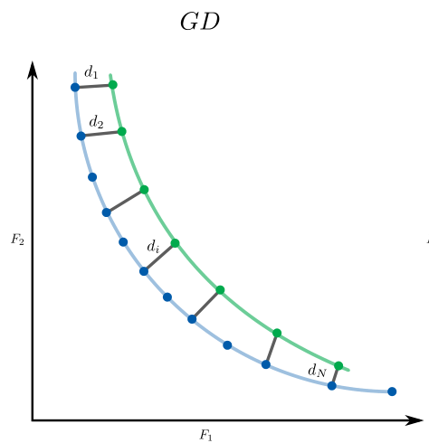
Metaheuristics.PerformanceIndicators.gd — Function

gd(front, true_pareto_front; p = 1)

Returns the Generational Distance.

Parameters

front and true_pareto_front can be:

N×m matrix where N is the number of points and m is the number of objectives.
State
Array{xFgh_indiv} (usually State.population)

source

Generational Distance Plus

Metaheuristics.PerformanceIndicators.gd_plus — Function

gd_plus(front, true_pareto_front; p = 1)

Returns the Generational Distance Plus.

Parameters

front and true_pareto_front can be:

N×m matrix where N is the number of points and m is the number of objectives.
State
Array{xFgh_indiv} (usually State.population)

source

Inverted Generational Distance

Inverted Generational Distance in Julia

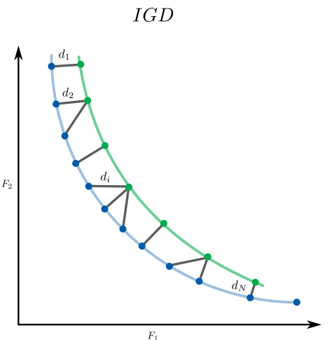
Metaheuristics.PerformanceIndicators.igd — Function

igd(front, true_pareto_front; p = 1)

Returns the Inverted Generational Distance.

Parameters

front and true_pareto_front can be:

N×m matrix where N is the number of points and m is the number of objectives.
State
Array{xFgh_indiv} (usually State.population)

source

Inverted Generational Distance Plus

Metaheuristics.PerformanceIndicators.igd_plus — Function

igd_plus(front, true_pareto_front; p = 1)

Returns the Inverted Generational Distance Plus.

Parameters

front and true_pareto_front can be:

N×m matrix where N is the number of points and m is the number of objectives.
State
Array{xFgh_indiv} (usually State.population)

source

Spacing Indicator

Metaheuristics.PerformanceIndicators.spacing — Function

spacing(A)

Computes the Schott spacing indicator. spacing(A) == 0 means that vectors in A are uniformly distributed.

source

Covering Indicator ($C$-metric)

Metaheuristics.PerformanceIndicators.covering — Function

covering(A, B)

Computes the covering indicator (percentage of vectors in B that are dominated by vectors in A) from two sets with non-dominated solutions.

A and B with size (n, m) where n is number of samples and m is the vector dimension.

Note that covering(A, B) == 1 means that all solutions in B are dominated by those in A. Moreover, covering(A, B) != covering(B, A) in general.

If A::State and B::State, then computes covering(A.population, B.population) after ignoring dominated solutions in each set.

source

Hypervolume

Hypervolume Indicator in Julia

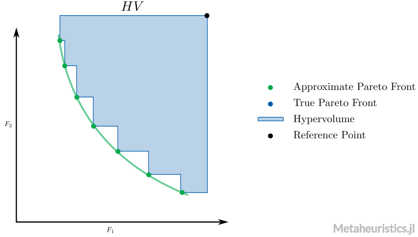
Metaheuristics.PerformanceIndicators.hypervolume — Function

hypervolume(front, reference_point)

Computes the hypervolume indicator, i.e., volume between points in front and reference_point.

Note that each point in front must (weakly) dominates to reference_point. Also, front is a non-dominated set.

If front::State and reference_point::Vector, then computes hypervolume(front.population, reference_point) after ignoring solutions in front that do not dominate reference_point.

source

Examples

Computing hypervolume indicator from vectors in a Matrix

julia> import Metaheuristics.PerformanceIndicators: hypervolume
julia> f1 = collect(0:10); # objective 1
julia> f2 = 10 .- collect(0:10); # objective 2
julia> front = [ f1 f2 ]11×2 Matrix{Int64}:
  0  10
  1   9
  2   8
  3   7
  4   6
  5   5
  6   4
  7   3
  8   2
  9   1
 10   0
julia> reference_point = [11, 11]2-element Vector{Int64}:
 11
 11
julia> hv = hypervolume(front, reference_point)66.0

Now, let's compute the hypervolume implementation in Julia from the result of NSGA3 when solving DTLZ2 test problem.

julia> using Metaheuristics
julia> import Metaheuristics.PerformanceIndicators: hypervolume
julia> import Metaheuristics: TestProblems, get_non_dominated_solutions
julia> f, bounds, true_front = TestProblems.DTLZ2();
julia> result = optimize(f, bounds, NSGA3());
julia> approx_front = get_non_dominated_solutions(result.population)        ⠀⠀⠀⠀⠀⠀⠀⠀⠀⠀⠀⠀⠀⠀⠀⠀⠀⠀F space⠀⠀⠀⠀⠀⠀⠀⠀⠀⠀⠀⠀⠀⠀⠀⠀⠀
        ┌────────────────────────────────────────┐
      2 │⠀⠀⠀⠀⠀⠀⠀⠀⠀⠀⠀⠀⠀⠀⠀⠀⠀⠀⠀⠀⠀⠀⠀⠀⠀⠀⠀⠀⠀⠀⠀⠀⠀⠀⠀⠀⠀⠀⠀⠀│ 
        │⠀⠀⠀⠀⠀⠀⠀⠀⠀⠀⠀⠀⠀⠀⠀⠀⠀⠀⠀⠀⠀⠀⠀⠀⠀⠀⠀⠀⠀⠀⠀⠀⠀⠀⠀⠀⠀⠀⠀⠀│ 
        │⠀⠀⠀⠀⠀⠀⠀⠀⠀⠀⠀⠀⠀⠀⠀⠀⠀⠀⠀⠀⠀⠀⠀⠀⠀⠀⠀⠀⠀⠀⠀⠀⠀⠀⠀⠀⠀⠀⠀⠀│ 
        │⠀⠀⠀⠀⠀⠀⠀⠀⠀⠀⠀⠀⠀⠀⠀⠀⠀⠀⠀⠀⠀⠀⠀⠀⠀⠀⠀⠀⠀⠀⠀⠀⠀⠀⠀⠀⠀⠀⠀⠀│ 
        │⠀⠀⠀⠀⠀⠀⠀⠀⠀⠀⠀⠀⠀⠀⠀⠀⠀⠀⠀⠀⠀⠀⠀⠀⠀⠀⠀⠀⠀⠀⠀⠀⠀⠀⠀⠀⠀⠀⠀⠀│ 
        │⠀⠀⠀⠀⠀⠀⠀⠀⠀⠀⠀⠀⠀⠀⠀⠀⠀⠀⠀⠀⠀⠀⠀⠀⠀⠀⠀⠀⠀⠀⠀⠀⠀⠀⠀⠀⠀⠀⠀⠀│ 
        │⠀⠀⠀⠀⠀⠀⠀⠀⠀⠀⠀⠀⠀⠀⠀⠀⠀⠀⠀⠀⠀⠀⠀⠀⠀⠀⠀⠀⠀⠀⠀⠀⠀⠀⠀⠀⠀⠀⠀⠀│ 
   f₂   │⡆⠀⠠⠤⠀⢀⡀⠀⠀⠀⠀⠀⠀⠀⠀⠀⠀⠀⠀⠀⠀⠀⠀⠀⠀⠀⠀⠀⠀⠀⠀⠀⠀⠀⠀⠀⠀⠀⠀⠀│ 
        │⡂⠀⠀⠁⠄⠀⢈⠄⠀⠢⠄⠀⠀⠀⠀⠀⠀⠀⠀⠀⠀⠀⠀⠀⠀⠀⠀⠀⠀⠀⠀⠀⠀⠀⠀⠀⠀⠀⠀⠀│ 
        │⠄⠀⠀⠐⠀⠀⠀⠀⠁⠀⠀⠂⠉⠠⠀⠀⠀⠀⠀⠀⠀⠀⠀⠀⠀⠀⠀⠀⠀⠀⠀⠀⠀⠀⠀⠀⠀⠀⠀⠀│ 
        │⠄⠀⠀⠈⠀⠀⠀⠈⠀⠀⠀⠁⠀⠀⠠⠑⡀⡀⠀⠀⠀⠀⠀⠀⠀⠀⠀⠀⠀⠀⠀⠀⠀⠀⠀⠀⠀⠀⠀⠀│ 
        │⠄⠀⠀⠐⠀⠀⠀⠈⠀⠀⠀⠀⠂⠀⠐⠀⠠⢐⡀⠀⠀⠀⠀⠀⠀⠀⠀⠀⠀⠀⠀⠀⠀⠀⠀⠀⠀⠀⠀⠀│ 
        │⡄⠀⠀⠐⠀⠀⠀⠁⠀⠀⠀⠁⠀⠀⠂⠀⠀⠄⡰⠀⠀⠀⠀⠀⠀⠀⠀⠀⠀⠀⠀⠀⠀⠀⠀⠀⠀⠀⠀⠀│ 
        │⠄⠀⠀⠐⠀⠀⠈⠀⠀⠐⠀⠐⠀⠀⠐⠀⠄⠀⠂⣕⠀⠀⠀⠀⠀⠀⠀⠀⠀⠀⠀⠀⠀⠀⠀⠀⠀⠀⠀⠀│ 
      0 │⡂⠀⢀⠁⠀⠀⡁⠀⢀⠈⠀⠀⢀⠂⢀⠈⡈⠁⡐⣢⡄⠀⠀⠀⠀⠀⠀⠀⠀⠀⡀⠀⠀⠀⠀⠀⠀⠀⠀⠀│ 
        └────────────────────────────────────────┘
        ⠀0⠀⠀⠀⠀⠀⠀⠀⠀⠀⠀⠀⠀⠀⠀⠀⠀⠀⠀⠀⠀⠀⠀⠀⠀⠀⠀⠀⠀⠀⠀⠀⠀⠀⠀⠀⠀⠀⠀2⠀
        ⠀⠀⠀⠀⠀⠀⠀⠀⠀⠀⠀⠀⠀⠀⠀⠀⠀⠀⠀⠀f₁⠀⠀⠀⠀⠀⠀⠀⠀⠀⠀⠀⠀⠀⠀⠀⠀⠀⠀⠀⠀
julia> reference_point = nadir(result.population)3-element Vector{Float64}:
 1.5067041421979686
 1.0034984531742384
 1.0012049665804095
julia> hv = hypervolume(approx_front, reference_point)0.9147903170937487

$\Delta_p$ (Delta $p$)

Metaheuristics.PerformanceIndicators.deltap — Function

deltap(front, true_pareto_front; p = 1)
Δₚ(front, true_pareto_front; p = 1)

Returns the averaged Hausdorff distance indicator aka Δₚ (Delta p).

"Δₚ" can be typed as \Delta<tab>\_p<tab>.

Parameters

front and true_pareto_front can be:

N×m matrix where N is the number of points and m is the number of objectives.
Array{xFgh_indiv} (usually State.population)

source

$\varepsilon$-Indicator

Unary and binary $\varepsilon$-indicator (epsilon-indicator). Details in E. Zitzler, L. Thiele, M. Laumanns, C.M. Fonseca, V.G. da Fonseca (2003)

Metaheuristics.PerformanceIndicators.epsilon_indicator — Function

epsilon_indicator(A, B)

Computes the ε-indicator for non-dominated sets A and B. It is assumed that all values in A and B are positive. If negative, the sets are translated to positive values.

Interpretation

epsilon_indicator(A, PF) is unary if PF is the Pareto-optimal front.
epsilon_indicator(A, B) == 1 none is better than the other.
epsilon_indicator(A, B) < 1 means that A is better than B.
epsilon_indicator(A, B) > 1 means that B is better than A.
Values closer to 1 are preferable.

Examples

julia> A1 = [4 7;5 6;7 5; 8 4.0; 9 2];

julia> A2 = [4 7;5 6;7 5; 8 4.0];

julia> A3 = [6 8; 7 7;8 6; 9 5;10 4.0 ];

julia> PerformanceIndicators.epsilon_indicator(A1, A2)
1.0

julia> PerformanceIndicators.epsilon_indicator(A1, A3)
0.9

julia> f, bounds, pf = Metaheuristics.TestProblems.ZDT3();

julia> res = optimize(f, bounds, NSGA2());

julia> PerformanceIndicators.epsilon_indicator(res, pf)
1.00497701620997

source